Overview
Questions of interest:
- What are the most important factors contributing to a person’s happiness?
- Do any specific regions to be happier than others?
This project was based on Kaggle’s World Happiness Report Dataset found here.
To supplement this analysis a Tableau Dashboard was created to help visualize region and country happiness for each year.
Explore Data
Load Data
Kaggle provides csv files for the years 2015 to 2019. Pandas can be used to load each year’s csv file.
2015 example below:
df15 = pd.read_csv('2015.csv')
Cleaning
Once the datasets have been loaded, it appears the data structure is different for 2017, 2018, and 2019. Any dataset-specific variable creation can be done before merging all datasets. For years 2017 to 2019, the ‘Region’ column has not been given. This will be important for visualizations and may be considered for the model. We can use the Country-Region pairs from 2015 to see if we can impute this column. A simple function was made:
region = df15.set_index('Country').to_dict()['Region']
def find_region(df):
    try:
        df['Region'] = region[df['Country']]
    except KeyError:
        df['Region'] = np.nan

    return df
This function can be applied to 2017, 2018, and 2019 data frames.
2017 Example:
df17 = df17.apply(find_region, axis = 1)
To determine the results of our imputation, we can consider how many NaN values are in the ‘Region’ column.
print(df17.isna().sum())
There are 6 missing ‘Region’ values. The datasets will be merged and then these missing regions will be filled.
Combine Datasets
The datasets can now be concatenated.
frames = [df15, df16, df17, df18, df19]
df_all = pd.concat(frames)
It is important for this analysis to not drop the rows with a missing ‘Region’ column. Because there are only 19 missing values, these regions will be manually input (Chances are they are similar across 2017, 2018, and 2019). To determine which countries are missing a region we can loop through each country.
result = df_all[df_all['Region'].isnull()].index.tolist()
for val in result:
    countries = df_all.iloc[val]['Country']
    countries = countries.splitlines()
    addition = {key: None for key in countries}
    print(addition)
The values in the addition dictionary can be filled and then added to corresponding rows in the combined dataset.
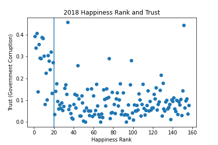
When considering the missing values in numeric columns, there only appears to be one for the ‘Trust’ column for 2018. From the plot below it appears, given the missing row was rank 20, the mean for the entire year is the best imputation.

EDA
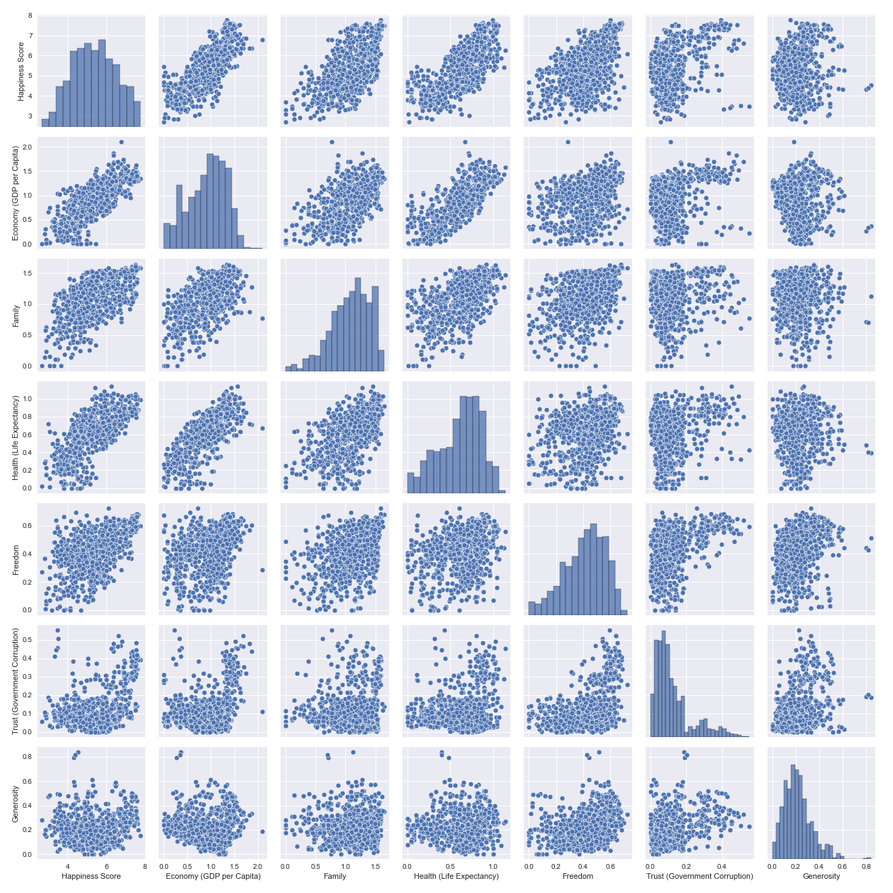
Once the data is cleaned, exploratory data analysis can be done to get a better understanding of the data. A pairs plot can be created to get an idea of the distribution of each variable and inspect multicollinearity.

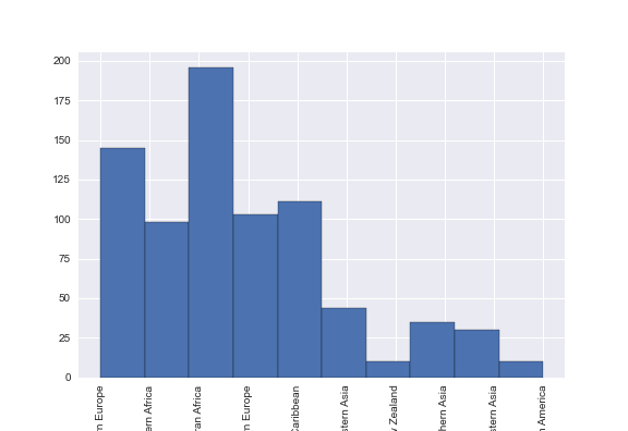
Next, we can consider the distribution of regions.

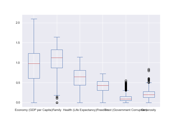
We can see that each country is not represented equally in the dataset. We must consideration this during preprocessing. For each predictor, a boxplot can give insight into the 5 number summaries of the data.

Preprocess
From EDA, there are a few preprocessing steps that must be done before exploring models. Three preprocessing steps were considered in this analysis.
Stratify Split
When creating a train and test set it is important the stratify on Region because the frequencies are not equal across all Regions.
train, test = train_test_split(happy_df, test_size=0.25, stratify=happy_df['Region'])
This will allow a model to be trained on a dataset that is more representative.
One Hot Encode
The two categorical variables, Region and Year, must be encoded.
train = pd.get_dummies(data=train,columns=['Region','Year'])
Normalize
From EDA, it is known the scales and range of each predictor variable are relatively similar. For this reason, it may not be necessary to normalize the predictors before fitting a model. Normalization may later be considered when exploring models.
Model
Note: Model building took place in R
To better understand what specific factors contribute to one’s happiness, regression techniques can be used.
Full Model
When building a model, we will consider all variables because it is not known which variables will best explain the Happiness Score. The full model will be specified as follows:
fit_full <- lm(`Happiness Score` ~ ., data = train_df)
summary(fit_full)
This model is a good start but the data may be able to be explained with a simpler model. Another thing we want to consider is the importance each feature plays in predicting happiness. The full model does not give us this information.
Regularization with Elastic Net
Using regularization methods, we are able to shrink less important coefficients to (or close to) zero. This will help with feature importance as well as possibly determining a simpler model.
In this case, elastic net can be used. Cross-validation can be used to determine the best value for λ (the penalty constant) and α (α: [0,1] where 0 = Ridge, 1 = Lasso). Because regularization methods are being used, the data will be centered and scaled before a model is fit. Elastic net can be fit using the “car” package in R; 5-fold cross-validation can be used.
set.seed(123)
control <- trainControl(method = "cv", number = 5) # 5 fold CV
elastic_fit <- train(`Happiness Score` ~ .,
                data = selected_vars,
                method = "glmnet", #specify elastic net
                preProcess = c("center", "scale"), #Preprocess: center and scale
                trControl = control)
To determine our optimal parameters:
elastic_fit$bestTune

Output:
    alpha     lambda
    0.1       0.01771384
The final model coefficients:
coef(elastic_fit$finalModel, elastic_fit$bestTune$lambda)

Output:

                                              s1
(Intercept)                           5.39134812
`Economy (GDP per Capita)`            0.40820405
Family                                0.31910350
`Health (Life Expectancy)`            0.18009433
Freedom                               0.17677472
`Trust (Government Corruption)`       0.10875080
Generosity                            0.08688597
`Region_Australia and New Zealand`    0.03449934
`Region_Central and Eastern Europe`   .
`Region_Latin America and Caribbean`  0.17692684
`Region_North America`                0.05179696
`Region_Southeastern Asia`           -0.07451232
`Region_Sub-Saharan Africa`          -0.06211095
Year_2015                             0.09169874
Year_2016                             0.17172231
Year_2017                            -0.02549139
Model Evaluation
To evaluate the final model we can consider the squared root of the mean squared error (RMSE).
#Predicted values
test_pred_en <- predict(elastic_fit, test_df)
#Actual values
test_act_en <- test_df$`Happiness Score`
#RMSE
rmse_en <- RMSE(test_act_en, test_pred_en)
rmse_en

Output:
0.527372
Conclusion
To expand on this study, other models can be evaluated and compared to the model fit above. We can conclude that the most important factor (from those in this dataset) in determining one’s happiness is the GDP per Capita of a country. When considering region, the Latin America and Caribbean region is the most important in determining one’s happiness (typically higher in comparison with other regions).